
1.- Introduction
The automatic analysis of ligand screening experiments requires several conditions to be met, not only the reprocessing must be performed in optimal conditions of phase and baseline correction, but the data ought to be correctly referenced and aligned.
2.- Preparation of reprocessing templates for each type of experiment.
In order to prepare the data to identify for the optimum reprocessing parameter, first we need to open each individual experiment, to do so effectively we will use the 'Multi-open' script, which can be found in the menu 'Scripts/Import/Multi-open where you should see something like:
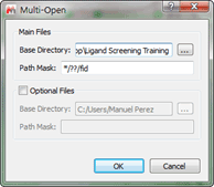
Figure 1
Next we need to point the script in the right direction so it will open only those spectra we desire, note that all the directories have a similar same structure: &,nbsp,
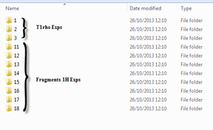
Figure 2 Directory structure
&,nbsp, We can see that all of the T1rho experiments are on folders 1-3 and the individual fragments on folders 11 and up. Hence in order to map the data and be able to open both types of experiments separately we will have to use the following file masks:
- For T1rho: */[1-2-3]/fid
- For Fragments: */??/fid
When we open either set, we will end up with several tens of spectra on our document, what we need to do next is to select all experiments on the page window (just click on the window as us ctrl-A) then press the stack button ![]() Â , the end result should look something like:
 , the end result should look something like:
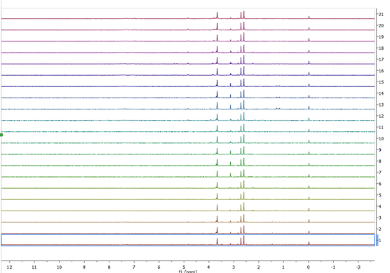
Figure 3 T1rho stacked spectra
Now we need to increase the intensity of all spectra, to do so we can either use the mouse wheel or the “+†and†–“ keys, the reason performing this step is to be able to monitor the changes that occur when using different processing functions are applied. For the set of T1rho experiments we are going to use the following reprocessing parameters:
- Blind region between 4.5 and 5.1 ppm, save this blind region, we will use this later:
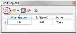
Figure 4 Blind Region Menu
- Use as phase correction algorithm “Globalâ€:
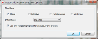
Figure 5 Phase Correction Options
Set baseline correction to “Polynomial Fit†with order 5:
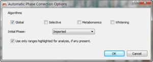
Figure 6 Baseline Correction Options
&,nbsp,
- Save the reprocessing template by going into the menu “Processing†>, “Processing Templateâ€, name the file T1rho Reprocessing
- Last go into blind regions >, “Edit Predefined Rules†and set the previously saved blind region as you choice for all 1H spectra
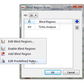
Figure 7 Blind Regions Rules
Next, we are going to perform the same procedure as above but now for the spectra of the individual fragments: Import all of the individual spectra using the Multi-Open script with the file mask “*/??/fidâ€
- Stack the spectra just opened
- Phase correct all spectra using “Whitening†algorithm
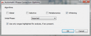
Figure 8 Phase Correction Options for Individual Fragments
- As above perform baseline correction by using the “Polynomial Fit†algorithm, order 5:

Figure 9 Baseline Correction Options for Individual Fragments
- Save this reprocessing template with the name “Fragments_Repâ€, remember go to “Processing†menu >, “Processing Templateâ€
At this stage we should have optimized the reprocessing of both types of experiments. Note: Experiment with the different phase and baseline correction algorithms so the benefits and limitations for each one of them becomes apparent, i.e. Whittaker baseline correction is very aggressive and effective, but note the loss of signal toward the end of the peaks.
3.- Data mapping
We are now in condition to start the data mapping, the process is analogous to the data importing step we performed above, but with one exception, now we will have to tell the software what every experiment means. To begin using the screening module, open the 1H NMR Screen from the Advanced Menu: 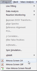 You will be presented with the main Project Info window:
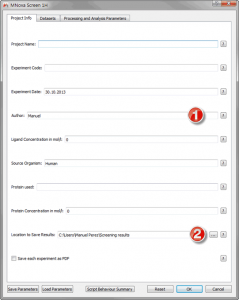
Figure 10 Project Info Tab
Of importance on this tab are the Author and the Results fields, the former will be used on your results files and the folder containing those experiments will be name with the date/time of the analysis followed by “_Authorâ€. The results location is where all the data which is produced by Mscreen will be saved. The rest of fields are at the present moment only used for information purposes . Next we will need to map our data and indicating the software exactly what each experiment is, in order to start doing so move to the “Datasets†tab:

Figure 11 Datasets Tab in Mscreen
There are three distinctive regions, the Project data region, where we will be mapping the screening experiments, the experiment region where we will indicate the software the nature of each experiment as well as the contents of the sample and finally the Reference data region where we will map each one of the individual fragments. In this current example we will use a direct way of mapping the data but there are additional methods to do so, for more information on this regard please read Mscreen manual. The first of steps will be to map the Project Data, in our case this will consist of three different T1rh experiments, in order to do so we will follow these steps:
- Navigate to the directory where the data is saved by clicking onÂ

- On the “Experiment Folder Pattern†we will use the following path mask “*/[1-2-3]/fid “, without the commas, you should now see this on your experiment window:

Figure 12 Initial Experiment Window
We will need to change the Types and Contents to the correct ones, so they will look something like:
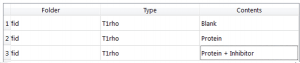
Figure 13 Final Values for Types and Contents
We shall now proceed at making our references, in order to do so, do navigate to the reference data folder by clicking , in this case we will use the following file mask “*/??/fidâ€. After mapping the reference data we should see a scene identical to the one depicted on Figure 11, where all the references have been associated to the corresponding experiments, as we can see in better detail on Figure 14.
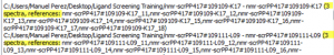
Figure 14 References Mapped to Project Data
4- Data Processing and Analysis
The next objective will be to set optimum parameters for the reprocessing and analysis of our screening data, we will be only detailing the conditions for T1rho type experiments. In order to set the scene the changes that will be monitoring are those occurring on the values of the integrals for different peaks. We will not be detailing in this document the theory behind the interactions taking place, for a thorough description please refer to “Progress in Nuclear Magnetic Resonance Spectroscopy 44 (2004) 225–256â€. At this stage is worth mentioning that for every option dialogs detailing what each one achieves has been created and you can access this by clicking on the question mark  ![]() buttons. Initially we will be presented with the tab, which will look like:
buttons. Initially we will be presented with the tab, which will look like:

Figure 15 Processing and Analysis Parameters
We will start by defining when we would like a peak to be considered a hit, this can be set under:
Figure 16 Condition for Hit
This value shown in Figure 16 will much depend on the system under study as well as the experience of the scientist, for the case of T1rho experiments setting a 25% as the condition for a hit is a good compromise (please note the “Optimise†button which can be used in this case to produce any number of analysis with different area percentage change conditions). We need to set the reprocessing parameters for the T1rho experiments, in order to start doing so click on the “Edit†button and the following panel will be presented in front of us:

Figure 17 T1rho Reprocessing Parameters
First we are going to set the normalization factor, in our case we will use the TSP peak around 0.0 ppm region – what this is going to enable is a consistent way to compare the changes that occur between the different experiments. The options we will use will be to normalise peaks by area and to use those peaks between -0.2 and 0.2 ppm.
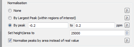
Figure 18 Normalisation Parameters for T1rho
Next we will proceed to define the alignment parameters as shown below:

Figure 19 Alignment Parameters
It is worth mentioning at this stage that most of the failures on the automatic analysis arise from the lack of good alignment in between samples, so consider this when examining data. In the “Processing Template†dialog navigate to the reprocessing template which was created early on. The noise/Impurity peak reduction will greatly depend on the quality of your data, but using a 5% of maximum peak is a reasonable general value. The settings for reference spectra will be identical to those we set for T1rho experiments, with the exception of the specific reprocessing template, hence make sure that your options look something like:

Figure 20 Processing Settings for Reference Spectra
We will set next the “Minimum matched peaks to be presentâ€, what this option does is to define how many peaks the software needs to match in the mixture to mark a reference sample as present in solution. This option is very useful when we an individual fragment has not been solvated and it is not in the mixture. We will set up this value at 10%:
Figure 21 Percentage of Matched Peaks
Next the Tolerance for matching peaks will be set, this particular value, this will be multiplied by the width at half eight of each peak and this will be the interval to the right and left of every peak which will be used to find a matching peak. Note that the higher we make this value the higher we will make the chance of mismatching a set of peaks, and the lower it is the more peaks we might miss in the matching process. The option of “Use Blank STD and T1rho peak matching to identify missing references†will have to be ticked in this particular example since for this dataset a scout experiment was not acquired. We have to define the spectral areas over which we wish to focus the automatic analysis, you can add as many areas as you wish, always being careful that there are not peaks that could interfere with the analysis (e.g. buffer or residual solvent peaks). In this particular dataset we will focus on the aromatic region between 6 and 13 ppm. Finally do not forget to save your parameters, check the “Script behavior summary†and click ok. After a few minutes running we will presented with a brief synopsis of the findings from the software:
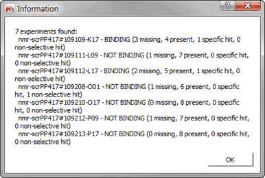
Figure 22 Results Briefing
Press OK and the results viewer should now be in front of you, it should look something like:

Figure 23 Results Editor
If we wish to review the results for any particular experiment we just need to double click on the experiment and the results will be brought on the main window. Before continuing it is worth detailing the four different states that can be attributed to one sample: -Â Â Â Â Â Â Â Â Â Present (yellow): Indicates that the compound has been found but it does not interact with the protein -Â Â Â Â Â Â Â Â Â Missing (red): no compound signals were found in the region of interest -Â Â Â Â Â Â Â Â Â Specific hit (blue): the compound shows interaction in the sample which contains the protein but not on the sample with protein and competitor -Â Â Â Â Â Â Â Â Â Non-selective hit (green): the compound shows interaction in both the sample which contains the protein and on the sample with protein and competitor If we click on the first of experiments we should see something like:
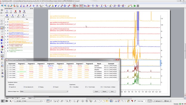
Figure 24
Trick: if you would like to manipulate individual spectra you can do so through the “Stacked Spectra Tableâ€, this is accessible from the “View†menu >, “Tablesâ€. Now we can start reviewing the data, the best way to do so is to focus on those samples which show hits or non-specific hits. To do so, just click on one of the samples, first one for examples and from the screening results editor untick present and missing:
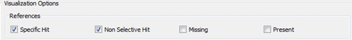
Figure 25
Superimpose the spectra by going into the stacked button:

Figure 26
In this manner we can very quickly review the hits, for example for the first of samples we can see by doble clicking through the stacked spectra table:

Figure 27 Visual analysis of a selective hit
The effect that we can see is how the intensity of the signals of interest for this particular fragment decrease in the presence of the protein under study and how when adding a competitor these recover, fullfilling the conditions for a selective hit. We can also use the results editor to examine the results in a more quantitative manner by using the pull-down menu “Reference Display Text†and selecting the appropriate metric:
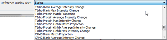
Figure 28
For example display T1rho Protein Average Intensity Change:
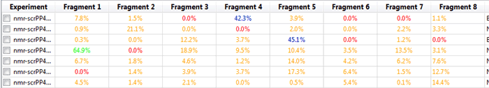
Figure 29
In this manner we can notice those fragments that might be close at being considered hits under our criteria. Furthermore, it is possible to create full reports with a combination of all of the metrics that Mscreen calculates and export these into .csv format by pressing the “Export†button, after doing so and opening for example on Excel we should see something like:
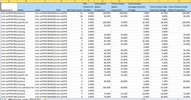
Figure 30 Results of Analysis
This will allow further analysis of the data in alternative ways.

