
A quiet revolution is occurring in the world of quantitation: qNMR. [1] I have written extensively on the subject in this blog [2], and there are many excellent peer-reviewed articles to consider. The big attractions for analysts are speed and convenience. You do not need to determine a response factor for every new compound, and your accuracy may be limited by your weighing skills. Furthermore, your analysis will equally apply to single compounds as well as mixtures.
For some applications, such as forensics, the highest levels of accuracy and precision are required, and a number of studies have shown that careful qNMR is well up to the task. [3] But in this case the technique becomes less of a high throughput method.
However you do qNMR, a huge part of the achievable accuracy and precision will depend on the signal integrations.
In this article I would like to look at integration in a little more detail, and show some of the steps needed for best practice. How far you wish to push qNMR depends on your attention to detail in this regard, so please read on – even if you don’t really want a “black belt” in integration! Note that there is already some good articles on integration and overlap. [4]
Line-shape
In these days of gradient shimming it can be easy to forget that the very best line-shape is a prize that still must be earned. Much of what you may ever want to do with NMR experimental data will be predicated on inherent signal line-shape. To assess you and your spectrometer performance it may be necessary to collect a spectrum that really shows how good your inherent line-shape is. I will speak to signal acquisition below, but assuming you have everything right, you can see my point, below.
Try the quick test to check your instrument’s line-shape: apply line fitting to a nice, clean singlet resonance having good signal-to-noise-ratio (SNR). Given that the algorithm assumes that your signal line-shape is pure Lorenzian, Gaussian, or a mix of both, this is a good check. Be sure to look at the signal at the very base of the peak: peak broadening there is quite common.
The spectrum, below, is of caffeine in DMSO-d6. The real data line is coloured black, the simulated line is purple, and the residual between the two is coloured red. You see that the line is poorly modelled at the base of the peak. If we add the integrals of the peaks in the region we determine the total integral to be 4437. If, however, we perform a standard integration (Sum) between 3.5 and 3.1 ppm, the absolute integral is shown to be 4080. The area overestimation and apparent integral error caused by an attempted line-shape analysis of an imperfect peak is therefore 8.75%, assuming Sum integration to be a correct determination.

What other consequences of poor line-shape are there?
There are many cases when you may wish to use a form of line fitting for quantitation (see below). For example, wide lines can make it more difficult to select the full region you need for accurate integration, because you are likely to be bumping into other signals. However, having asymmetric lines or a hump under the peak just means that any line-shape simulation you may wish to attempt will give an erroneous result.
Spectrum acquisition: use a long acquisition time?
A lot has been said about the considerations when acquiring data for accurate quantitation – and justifiably so. After having looked at a lot of external data I would add one item to the list: avoid truncation artefacts by using a long acquisition time. Why not acquire 128K or 256K data points? Yes, this will adversely affect the final signal-to-noise-ratio (SNR), but I am assuming that you are not sample limited. If you do this then you will be less reliant on apodisation functions to force the signal intensity to zero at the end of the acquisition period, the common way to suppress truncation artefacts.
Some users acquire a 1H NMR spectrum with a short acquisition time, and then try to reclaim decent digitisation using forward Linear Prediction (fLP). This is not a wise strategy, as fLP really works best when there are just a few signals (“coefficients”) – as is the case with 2D data. It is better just to collect a FID having lots of data points, and shorten the relaxation delay accordingly. The total experiment time is unaffected.
There is a measure of personal preference in this recommendation, and many spectra are acquired without the consideration. I advocate collecting as near to a perfect signal as possible from the sample.
Data point resolution
In much of the discussion that follows, it will become apparent that the number of data points that are used to describe an NMR peak will clearly have a significant impact on the integration fidelity. Rather than just considering the point-to-point distance (Hz), it is worthwhile looking at the number of data points that describe the peak, as this will ultimately impact on any integration method.
Classical integration
We use classical (“Sum”) integration every day, but how is this performed with digital data? I can do no better than refer you to an excellent blog on the subject [4], but the basic approach is to approximate the signal to a series of rectangles, and sum those areas. It’s simple but effective.
In the spectrum, below, you see a schematised depiction of the process. The data points are shown as maroon crosses, and the software will determine the area of the peak from the sum of areas of the yellow rectangles it silently determines.

A poorly-digitised peak can only lead to a higher inaccuracy in the Sum integral.
Global Spectrum Deconvolution (GSD)
Whilst GSD [5] is not as complete as classical line fitting, it is an extremely fast algorithm. Hundreds of lines in a spectrum can typically be fitted in a few seconds. GSD determines line position (frequency), width, and height, and a "shape" parameter (kurtosis) using its proprietary fitting algorithm. (Kurtosis is is similar to the Lorentzian/Gaussian factor, yet mathematically different.) From these data the integral for each peak is calculated. For many, GSD is the default peak analysis method used to report peak positions and absolute integrals.
The Mnova user can choose whether to use the GSD or Sum method to determine absolute integrals: this is a key consideration in qNMR.
So, how do the methods compare?
Signal overlap
Where signal overlap is an issue, GSD is highly favoured. If you look at the spectrum of estradiol in DMSO-d6, below, you see that the H-12 triplet cannot be accurately integrated (lower trace) because of overlap with the broad water signal. GSD correctly determines the properties of the triplet peaks and broad, overlapping signal, and this is better seen in the extracted “spectrum” (upper trace) of the compound alone. GSD will provide an integral just of the triplet.

Integration accuracy
As mentioned previously, integration is at the heart of qNMR. So, are integrals derived from GSD and Sum equally accurate and precise? In the test, below, I show a spectrum of felodipine in DMSO-d6 solvent, with 8 multiplet regions selected. If we determine the normalized integrals by dividing by the number of nuclides, the integration value for all regions should be equal, within experimental error.

In the table I have summarized the result of this analysis for the cases where I used Sum and GSD integrals. The average of the 8 values and RMSD is shown.
| Sum | GSD | |
|---|---|---|
| Average | 36298.7 | 38086.4 |
| Standard dev (%) | 0.53 | 2.90 |
We see that integrals derived from GSD show a significantly higher standard deviation than those from Sum integration, and this is a typical result. The error for GSD is still acceptable for all but the most demanding integration determinations, and is commonly used in Mnova.
GSD-derived integrals will probably be of sufficient accuracy and precision for many applications, particularly those involving mixtures. But for “ultra high-precision qNMR”, Sum integration should be used wherever possible.
Edited Sum integration
This topic will be discussed in detail in a forthcoming publication. [6] This integration method is a hybrid of Sum and GSD integration, and will be of interest to those seeking the most accurate integration/quantitation result.
The idea is to use Sum integration of peaks, and a wide integral width throughout the spectrum. Low-level impurities, however, can inevitably cause inaccuracies if they lie in the integration limits. Although the Sum integral of the low-level impurities cannot be accurately determined due to insufficient SNR, the GSD-derived integration of the impurities are quite accurately determined. So the method relies on subtraction of GSD integrals of impurities from the Sum integral of the region.
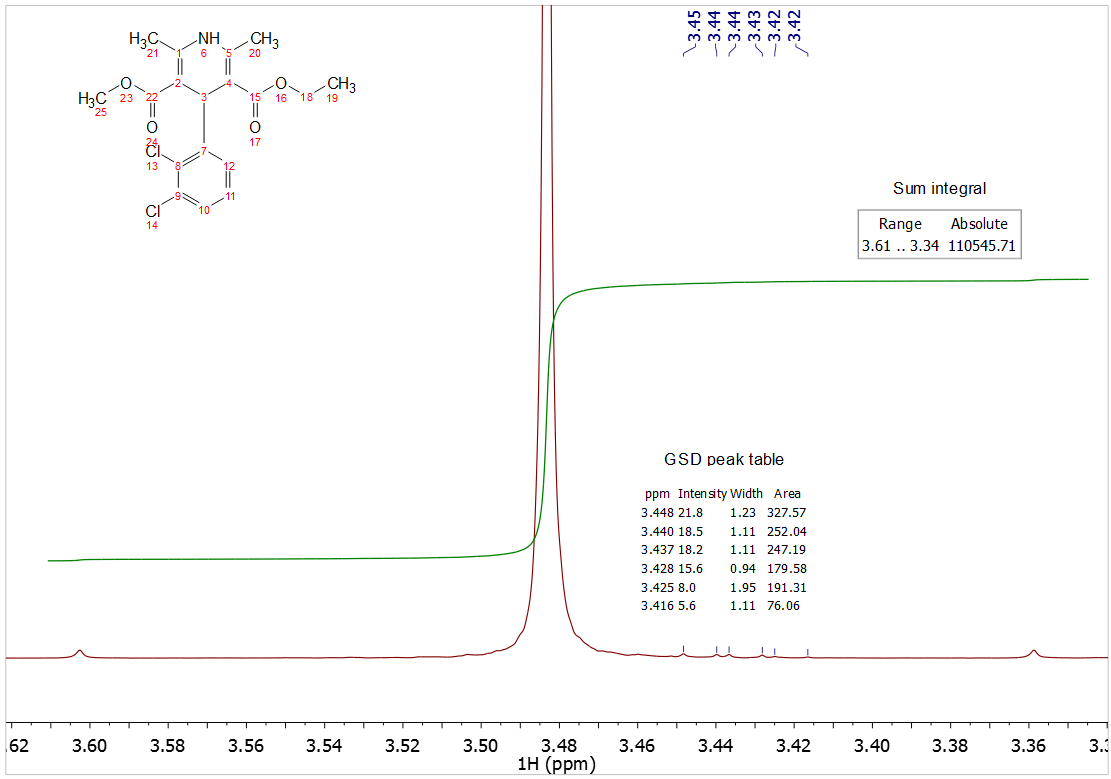
The most accurate integral for this region would therefore be:
110545.7 – (327.6 + 252.0 + 247.2 + 179.6 + 191.3 + 76.1)
= 109271.9
Sensible integral regions selection for qNMR
Fundamental to qNMR in Mnova is the ability to select the regions that will contribute towards the most accurate result. With the qNMR plugin there are sophisticated “rules” that the user can specify the software to consider, such as ignoring labile protons, disfavouring singlets, etc. In practice, it is often sufficient to ask the software to automatically select multiplets that produce a result having the smallest RMSD.
The latter will likely cause the software to do what you would do yourself, by disfavouring the selection of “contaminated” multiplets for quantitation. Common sources of contamination will be residual solvents, degradation products, impurities, etc.
Conclusions
The use of high-resolution NMR for compound quantitation is a powerful technique. We see that signal integration is at the heart of its applicability and accuracy, but options exist to make the technique as reliable as is needed.
Acknowledgement
I would like to thank Dr Carlos Cobas for valuable input into this article.
References
- Simmler, C., Napolitano, J. G., McAlpine, J. B., Chen, S.-N., & Pauli, G. F. (2014). Universal quantitative NMR analysis of complex natural samples. Current Opinion in Biotechnology, 25, 51–9. doi:10.1016/j.copbio.2013.08.004
- https://resources.mestrelab.com/qnmr-purity-recipe-book-i/; https://resources.mestrelab.com/qnmr-purity-recipe-book-ii/; https://resources.mestrelab.com/nmr-quantification/; https://resources.mestrelab.com/qnmr-of-mixtures-what-is-the-best-solution-to-signal-overlap/
- Schoenberger, T. (2012). Determination of standard sample purity using the high-precision 1H-NMR process. Analytical and Bioanalytical Chemistry, 403(1), 247–54. doi:10.1007/s00216-012-5777-1
- http://nmr-analysis.blogspot.com.es/2009/11/basis-on-qnmr-integration-rudiments.html; http://nmr-analysis.blogspot.com.es/2010/01/basis-on-qnmr-integration-rudiments.html; http://nmr-analysis.blogspot.com.es/2010/01/on-integrating-overlapped-peaks.html
- Bradley, S. a, Ouyang, A., Purdie, J., Smitka, T. a, Wang, T., & Kaerner, A. (2010). Fermentanomics: monitoring mammalian cell cultures with NMR spectroscopy. Journal of the American Chemical Society, 132(28), 9531–3. doi:10.1021/ja101962c; http://mestrelab.com/pdf/posters/Poster_2008_GSD.pdf
- Schoenberger and collaborators, manuscript in preparation.

 and Mestrelab Research, S.L. (Mestrelab)")
