
Introduction
Since the very first release of Mnova, we have been (and still are!) very fortunate to include in the software the prediction of NMR spectra provided by Modgraph Consultants. It is really a privilege to offer prediction capabilities developed by the pioneers and leaders in the field for so many years. Nowadays, when Machine and Deep Learning techniques are so popular, it is worth remembering that the predictions commercialized by Modgraph have used Neural Networks (in addition to other methods, vide infra) for more than 25 years already.
Modgraph pioneered the concept of combining several NMR prediction methods (see, for instance http://www.modgraph.co.uk/Downloads/TD_20_1.pdf) . For example, in the case of 13C Prediction, Modgraph combines a Neural Network prediction with the so-called HOSE prediction (http://www.modgraph.co.uk/product_nmr_HOSE.htm), both developed by Professor Wolfgang Robien of the University of Vienna and recognized as to offer the most reliable C13 NMR predictions for many years. They have implemented a procedure that selects the "Best" C13 prediction for each atom from the two prediction methods (Neural Network + HOSE).
Based on the idea that different predictors can be combined to form a potentially better predictor, we have added more predictors in Mnova 14 which are combined (using a Bayesian approach) with two main objectives: (1) Improve overall prediction accuracy (2) Reduce the number of prediction outliers.
The need of an ensemble NMR Prediction
Leaving aside slow quantum mechanical (QM) calculations, usually by the gauge-invariant atomic orbital (GIAO), all fast NMR prediction methods use in one form or other databases of assigned data. In a nutshell, we can consider the following fast prediction approaches:
- Increments methods (look-up tables of fragments)
- HOSE-code methods
- Machine Learning methods
The first two methods perform quite accurately as long as the predicted atom is well represented in the internal data base.
However, no matter how large the database used, it is going to be extremely tiny compared to the actual chemical space (i.e. the universe of possible compounds). For example, there are more than 166 billion organic molecules up to 17 atoms of C, N, O, S, and halogens, sizes compatible with many drugs [1]. And if we consider larger molecules (e.g. MW up to 500), the best guess for the number of plausible compounds is around 1060. There is therefore an effectively endless frontier.
On the other hand, whilst Machine Learning (ML) methods are known to show a higher extrapolation/interpolation power, the accuracy of the prediction will nevertheless be compromised to some extent by the similarity of the chemical environment of the atom to be predicted as compared to the data set used to train the ML model.
In summary, the accuracy of these fast NMR predictors depends, to a greater or lesser extent, on the contents of the assigned database. And whilst there are very large databases such as those provided by Modgraph 13C NMRPredict, it will be impossible to cover the full chemical universe.
But what if different prediction algorithms, trained with different data sets, are used together? In principle, one might expect that any deficiency of one of the available predictors can be compensated by any of the other predictors. This could help not only to get more accurate predictions but also to reduce the number of prediction outliers where the predicted values were exceptionally poor for a particular individual predictor.
Actually, in the field of Machine Learning, the concept of combining multiple learning algorithms (e.g. classifiers) is quite popular and it is known as Ensemble Learning (https://en.wikipedia.org/wiki/Ensemble_learning ).
Ensemble NMR Prediction
Suppose that a chemical shift has been estimated by several ‘predictors’ and that each estimator can characterize in some way the ‘reliability’ of its own estimate (i.e. prediction confidence interval).
How should one combine the various partial predictions and derive the statistical characteristics of the final outcome? This is a wide area of study, as there are many different special situations (contexts). A very naïve approach would consist in simply averaging the values. A weighted average using the confidence interval of each predictor would be probably a better approach. We have implemented a Bayesian mechanism that uses the information of the individual predicted chemical shifts (such as their distances) as well as their corresponding confidence intervals. A detailed description of the method is beyond the scope of this entry, but will be published elsewhere later.
The overall idea is illustrated in the figure below. Mestrelab and Modgraph predictions are executed in the background. Each predictor gives both chemical shifts (δ) and an estimate of its reliability (σ). Next, those individual values are combined together to yield a final chemical shift and reliability.

Figure 1: Combination of several individual predictors to yield a final prediction
In practice, this is how it works in Mnova. First of all, it is necessary to check the 1H or 13C Prediction options to ensure that different predictions are available. This might depend upon the licenses installed, but assuming that they are available, the options should look like this:
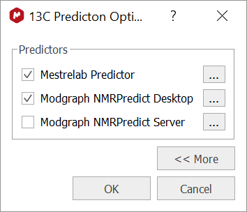
Figure 2: 13C Prediction options in Mnova 14
For the moment, Modgraph NMRPredict Server can be ignored. If the other two options are checked, when a prediction is issued, Mnova runs several predictors in the background. First, Mestrelab Predictor, which in fact, is formed by two different Machine Learning predictors (and both trained with different assigned data). Next, Modgraph Predictor is also executed (which in turn, uses two different predictors, vide supra). Finally, Mnova uses the Bayesian algorithm to combine all the individual chemical shifts and confidence intervals to yield the final predicted chemical shifts and confidence intervals.
As a result, Mnova will show the unified, final results, but it is possible to visualize the individual values for each predictor by inspecting the Mnova log file, although this will not be covered in this post.
Some results
To illustrate the benefits offered by the combination of several predictors a simple exercise has been conducted. A small set of 13 assigned molecules abstracted from the literature has been used. This was done by an internship student who had no knowledge about the contents of the Mnova prediction assigned DBs. In principle, the ideal set of molecules should be those that were not contained within the internal prediction DBs or used in the Machine Learning training sets. However, it was found that these molecules are actually pretty well represented in the internal DBs, as shown in Table 1. It can be seen that most of the Carbon atoms can be described by 4 or 5 shells. This is not a coincidence: it confirms the high quality (and huge size) of the Modgraph’s 13C HOSE DB!

Table 1: Distribution of number of shells for the molecules used in this test.
Nevertheless, bearing this point in mind, this small set of molecules should be good enough for this simple exercise. The overall results are summarized in Table 1.
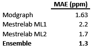
Table 1: Mean absolute errors for the individual and ensemble predictor.
First, it can be observed that the Mean Absolute Error (MAE) of Modgraph is remarkably low (1.63 ppm), reflecting the previous point that showed that most of the atoms in the test set are represented by 4 or 5 shells. The other two predictors (Machine Learning 1 and Machine Learning 2) also yield very good results, although slightly worse than Modgraph.
The question is: can those 3 predictors be combined in such a way that the result is better than all the individual predictors? That is the goal of the ensemble predictor and, as it is shown in Table 1, this is indeed the case: the ensemble predictor has a MAE = 1.3, a value which, in the context of 13C NMR prediction can be considered as exceptionally good.
Somehow, the ensemble predictor attempts to compensate any deficiencies of any of the individual predictors. For this to work, it is crucial that each predictor provides a reliable confidence interval and a very significant effort has been put into that.
Additional insights can be extracted by analyzing the histograms of the prediction errors for the individual and final ensemble predictors. They are shown in Table 3 and Figure 3.

Table 3: Distribution of prediction errors for the different individual predictors as well as for the final, ensemble result.

Figure 3: Histrogram plot corresponding to the data shown in Table 3
The most obvious conclusion that can be drawn from these histograms is that the ensemble method helps to group the prediction error around the low MAE zone and hence, reduce the number of large prediction errors. In other words, this method assigns a higher weight in the final prediction result to that prediction with a smaller confidence interval. However, it is important to bear in mind that this is an oversimplification as the Bayesian algorithm not only uses the confidence interval but also the distance in the predicted chemical shifts amongst the different predictors.
To complement this article, you can see some some results for 1H NMR data in the this blog post where a few assigned molecules were taken from the literature.
Bibliography
[1] J. Chem. Inf. Model., 2012, 52 (11), pp 2864–2875


 and Mestrelab Research, S.L. (Mestrelab)")